Soil risk assessment of heavy metal

Geostatistical analysis based on GIS

Indicator kriging

Spatial interpolation and GIS mapping techniques

The probability maps of soil Cr, Cd, Ni and Pb

were employed to produce spatial distribution and

concentration to exceed the respective FAO (2000)

risk assessment maps for the four observed heavy

maximum permissible limit value (MPL) of 100, 3,

metals, and the software used for this purpose was

30 and 50 mg kg -1 were prepared using indicator

ArcGIS v.9.3 (ESRI Co, Redlands, USA). The first

kriging. Indicator kriging is a nonlinear geostatistics

step was taking the log-transformation of all non-

where the conventional linear kriging estimators are

normally distributed target variables (heavy metal

applied to the data after a nonlinear transformation.

contents) to ensure (in most cases) the normality of

Here the nonlinear transform is to a discrete (binary)

residuals. In ArcGIS, kriging can express the spatial

indicator variable. These techniques have been

variation and allow a variety of map outputs, and

widely applied by soil scientists (Van Meirvenne and

at the same time minimize the errors of predicted

Goovaerts, 2001; Reza et al., 2012; 2013).

values. Moreover, it is very flexible and allows users

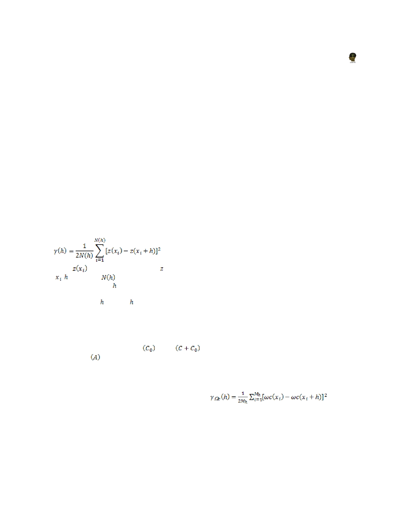
Let us assume that a soil property z at location x take

to investigate graphs of spatial autocorrelation. In

value z ( x ). In geostatistics, we treat this value as a

kriging, a semivariogram model was used to define

realization of the random function Z(x) . An indicator

the weights of the function (Webster and Oliver,

transformation of z ( x ) can be defined by

2001), and the semivariance is an autocorrelation

statistic defined as follows (Mabit and Bernard ,

ω _c ( x ) = 1

if z ( x ) ≤z _c ,

0 otherwise,

2007):

Where z is a threshold value of the property. In indicator

c

geostatistics, ω _c ( x ) is regarded as a realization of the

random Ω _c ( x ),

Ω _c ( x ) = 1

if z ( x ) ≤z _c ,

else 0.

where

is the value of the variable at location of

It can be seen that

,

the lag and

the number of pairs of sample

Prob [ Z ( x )≤ z ] = E [ Ω c ( x ) ] = G [ Z ( x ); z ] ,

c

c

points separated by . For irregular sampling, it is

Where Prob [ ] , E [ ] denote, respectively, the

rare for the distance between the sample pairs to be

probability and the expectation of the terms within

exactly equal to . That is, is often represented by

the square brackets, and G [ Z ( x ); z ] is the cumulative

c

a distance band.

distribution function of Z ( x ) at value z . The principal

c

Best-fit model with minimum root mean square

of IK is to estimate the conditional probability that

error (RMSE) was selected for each heavy metal.

z ( x ) is smaller than or equal to a threshold value

Using the model semivariogram, basic spatial

z _c , conditional on a set of observations of z at

parameters such as nugget

, sill

neighbouring sites, by kriging Ω _c ( x ) from a set of

and range

was calculated which provide

indicator-transformed data.

information about the structure as well as the

A set of data on z is transformed to the indicator

input parameters for the kriging interpolation

variable ω _c ( x ). The variogram of the underlying

(Dagar and Esfahan, 2013). Nugget is the variance

random function Ω _c ( x ) is then estimated by

at zero distance, sill is the lag distance between

measurements at which one value for a variable

does not influence neighboring values and range

Where M pairs of observations that are separated by

h

is the distance at which values of one variable

the lag interval h . A set of estimates of this indicator

become spatially independent of another (Lopez-

variogram at different lags may then be modeled by

Granados et al., 2002; Reza et al., 2010).

one of the authorized continuous functions used to

789