Dasyam et al.

Results and Discussion

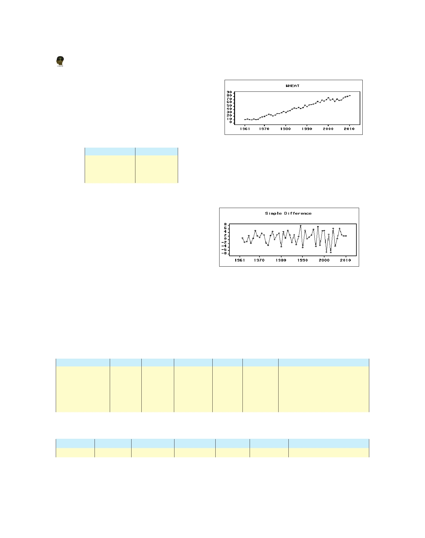
Atȱfirst,ȱwheatȱproductionȱdataȱinȱIndiaȱfromȱ1961-

2010ȱwasȱtestedȱforȱoutliersȱbyȱGrubbsȱmethod.ȱItȱwasȱ

observedȱthatȱtheȱnumberȱofȱextremeȱobservationsȱinȱ

theȱpresentȱdataȱwasȱzero,ȱasȱpresentedȱinȱTableȱ1.

Table 1. Grubbs test for detecting Outliers

Figure 1. Time series plot of wheat production

Mean:

44.6748

SD:

23.0635

ADFȱtestȱforȱunitȱrootȱalsoȱconfirmedȱthatȱtheȱdataȱ

wasȱnonstationaryȱandȱitȱbecameȱstationaryȱatȱfirstȱ

No of observations:

50

differenceȱasȱtheȱcalculatedȱvaluesȱwereȱlesserȱthanȱ

Outlier detected?

No

criticalȱvaluesȱatȱ1%,ȱ5%ȱandȱ10%ȱlevelsȱ(Tableȱ4).ȱItȱ

BeforeȱanalyzingȱbyȱARIMA,ȱparametricȱregressionȱ

isȱalsoȱclearȱfromȱtheȱtrendȱofȱtimeȱseriesȱplotȱatȱfirstȱ

andȱHoltȱmodelsȱwereȱappliedȱtoȱtheȱdatasetȱunderȱ

differenceȱasȱrevealedȱinȱFigureȱ2.

consideration.ȱFromȱTableȱ2,ȱitȱcanȱbeȱconcludedȱthatȱ

theȱQuadraticȱmodelȱwasȱsuperiorȱtoȱotherȱselectedȱ

regressionȱ modelsȱ basedȱ onȱ diagnosticȱ criteria.ȱ Itȱ

mightȱbeȱdueȱtoȱtimeȱseriesȱdataȱofȱwheatȱproductionȱ

followsȱquadraticȱgrowthȱpattern.

Similarly,ȱparametersȱofȱHoltȱmodelȱwereȱestimatedȱ

asȱlevelȱ(α)ȱ=ȱ0.539ȱandȱtrendȱ(β)ȱ=ȱ0.001ȱandȱdepictedȱ

inȱTableȱ3.

Figure 2. Time series plot for first differenced wheat

Afterȱconsiderationȱofȱtheseȱmodelsȱviz.ȱQuadraticȱ

production

andȱ Holt,ȱ ARIMAȱ techniqueȱ wasȱ employedȱ inȱ

addition.ȱAtȱ first,ȱ stationarityȱ ofȱ wheatȱ productionȱ

Afterȱfixingȱtheȱvalueȱofȱdȱasȱ1,ȱvaluesȱofȱpȱandȱqȱwereȱ

inȱ Indiaȱ fromȱ 1961-2010ȱ wasȱ testedȱ byȱ timeȱ seriesȱ

determined.ȱFromȱcorrelogramȱofȱACFȱandȱPACFȱasȱ

plotsȱ andȱ ADFȱ test.ȱ Theȱ timeȱ seriesȱ plotȱ clearlyȱ

shownȱ inȱ Figureȱ 3,ȱ thereȱ wasȱ onlyȱ oneȱ significantȱ

indicatedȱthatȱtheȱdataȱwasȱnonȱstationaryȱbecauseȱ

spikeȱforȱbothȱACFȱandȱPACFȱatȱlagȱ1.

ofȱprominentȱincreasingȱtrendȱasȱshownȱinȱFigureȱ1.

Table 2. Parametric regression models for estimation of wheat production

Model

R 2

RMSE

MAPE

MAE

MSE

Fitted Equation

Linear

0.968

3.381

8.653

2.625

11.433

Z _t = 4.775 + 1.564t + e _t

Quadratic

0.978

3.361

8.403

2.595

11.294

Z _t = 83.691 + 1.462t - 0.002t 2 + e _t

Exponential

0.826

9.513

16.642

6.915

90.512

Z _t = 2.525 Exp (0.043t) + e _t

Power

0.948

5.191

14.209

4.318

26.946

Z _t = 1.544 t 0.699 + e _t

Logarithmic

0.791

10.435

32.934

8.624

108.908

Z _t = -23.834 + 23.071 ln(t) + e _t

Table 3. Exponential Smoothing models for estimation of wheat production

Model

R 2

RMSE

MAPE

MAE

MSE

Estimation of Parameters

Holt

0.980

3.142

7.997

2.769

9.873

α= 0.539 , β=0.001

306