Temporal variation of rainfall trends in parambikulam aliyar sub basin, Tamil Nadu

Trend analysis

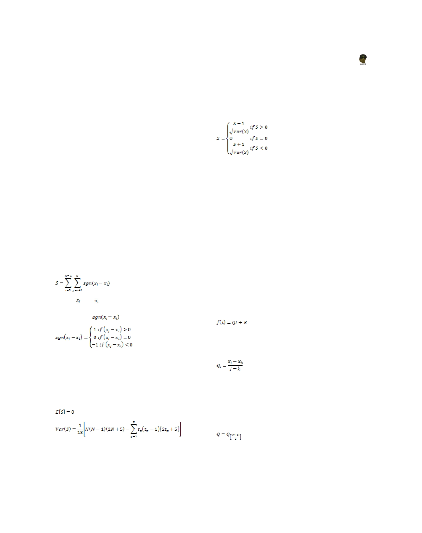
Here q is the number of tied (zero difference between

Thetrendanalysiswasdoneinthreesteps(Olofintoye

compared values) groups, and tp is the number of

and Adeyemo 2011). The first step is to detect the

data values in the pth group. The values of S and

presence of a monotonic increasing or decreasing

VAR(S) are used to compute the test statistic Z as

trend using the nonparametric Mann-Kendall test in

follows

the annual and seasonal rainfall time series, second

step is estimation of magnitude or slope of a linear

trend with the nonparametric Sen’s Slope estimator,

third one is to develop regression models.

Mann-Kendal test

The presence of a statistically significant trend is

evaluated using the Z value. A positive value of Z

The non-parametric Mann-Kendall test, which is

indicates an upward trend and its negative value

commonly used for hydrologic data analysis, can

a downward trend. The statistic Z has a normal

be used to detect trends that are monotonic but not

distribution. To test for either an upward or

necessarily linear. The null hypothesis in the Mann-

downward monotone trend (a two-tailed test) at α

Kendall test is independent and randomly ordered

level of significance, H0 is rejected if the absolute

data. The Mann-Kendall test does not require

value of Z is greater than Z1-α/2, where Z1-α/2 is

assuming normality, and only indicates the direction

obtained from the standard normal cumulative

but not the magnitude of significant trends (Mann

distribution tables. The Z values were tested at 0.05

1945, Kendall 1975).

level of significance.

The Mann-Kendall test statistic S is calculated using

the formula that follows:

Sen’s slope estimator

The magnitude of the trend in the seasonal and

annual series was determined using a non parametric

method known as Sen’s estimator (Sen 1968). The

Where and

are the annual values in years j and i,

Sen’s method can be used in cases where the trend

j>i respectively, and N is the number of data points.

can be assumed to be linear that is:

The value of

is computed as follows:

Where Q is the slope, B is a constant and t is time. To

get the slope estimate Q, the slopes of all data value

pairs is first calculated using the equation:

This statistics represents the number of positive

differences minus the number of negative differences

for all the differences considered. For large samples

(N>10), the test is conducted using a normal

Where xj and xk are data values at time j and k (j>k)

approximation (Z statistics) with the mean and the

respectively. If there are n values xj in the time series

variance as follows:

there will be as many as N = n(n-1)/2 slope estimates

Qi. The Sen’s estimator of slope is the median of these

N values of Qi. The N values of Qi are ranked from

the smallest to the largest and the Sen’s estimator is

, if N is odd

39